Introduction
Ever wondered what technologies are involved in making a VoIP phone call?
Fig 1 below is a pictorial view of the various stages of the signal flow in a typical VoIP phone. In this article we will start by examining why voice is digitized, the need for low pass filtering and the frequency it must be sampled at. We will then go on to look at advancements in communication theory and examine the use of Codecs. Finally, we will examine the protocols used to packetize the voice in a Voice over IP network and the resulting bandwidth required in transmitting speech. Also this article is aimed at users who have a fundamental understanding of Electronic Engineering principles.
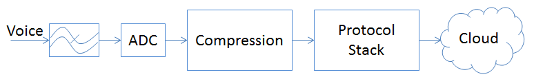
Figure 1: Voice Transmission Data Flow
First let�s look at why voice is sampled and digitized as opposed to just transmitting the analog voice.
Why Digitize?
Why digitize an analog signal?
The main reasons to digitize analog signals are:
- They are less susceptible to noise than analog signals
- They are easier to manipulate and transport around a communication network
- They can be checked for errors to ensure correct transmission
- Errors in transmission can be detected and corrected
The Digital revolution
When did the digital revolution begin?
When most people think of the digital world they think cell phones, smart phones, camcorders, cameras, etc. All of these products were introduced in the 1980's but they only really became mainstream in the 90's when they became affordable and available to the masses.
However, back in the mid 1960 there was a significant digital revolution going on - your home phone service. The Plain Old Telephony System (POTS) started to go digital. Most users were unaware of the changes as the physical phone remained largely the same but rather the voice was digitized further up the network which allowed the service providers and operators to realize the advantages of digital signals.
That revolution is continuing today as services such as VoIP, video calls, remote monitoring of you house, etc. become mainstream. We have come a long way in the last 50 years form having an operator physically switch your call to having the services we rely on today.
Process of Digitization
Regardless of where your voice is sampled, it could be in an IP phone or in the Analog Telephone Adapter (ATA) in networks that carry VoIP calls or digitized at the branch exchange in a POTS call, the process is identical.
How fast do you have to sample an analog signal?
The first parameter that has to be determined with any analog signal to be digitized, is how fast to actually sample it. To do this you must first determine the highest frequency you wish to sample. When having a conversation the typical frequency range of your voice is approximately 300-10000Hz. However most of the useful information to have a toll quality phone call is in the 100-3000Hz range. Fig 2 below shows the amplitude versus frequency response of a typical conversation.
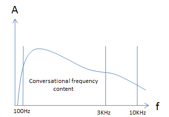
Figure 2: Unfiltered Speech Spectrum
The frequency content below approximately 100Hz and above 3000Hz adds very little to the quality of a phone call.
Sampling Theorem
One of the most important theorems in communication is the Nyquist - Shannon theorem. This theorem is the basis of all digital communications; it essentially states that the sample rate must be at least twice the highest frequency you wish to digitize to be able to accurately reconstitute the signal back into the analog domain. Thus, to digitize a typical conversation where all the useful information is in the 100Hz-3000Hz range, then we must sample at a minimum of 6000Hz. In the telecoms world we typically sample at 8000Hz, the reasons for this will become clear when we talk about filters.
First, let�s look at what a sampled signal looks like in the frequency domain. When a signal is sampled two things happen.
- The sampled signal is aliased to form a mirror image of itself around the sampling frequency.
- The sampled signal repeats itself at integer numbers of the sampling frequency.
Figure 3 shows a speech waveform that has been sampled at a frequency (fs) which is significantly higher than the maximum frequency content of the original analog signal.
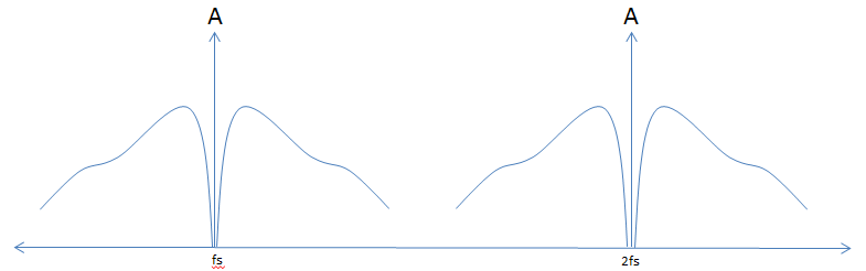
Figure 3: Sampled Unfiltered Speech Spectrum
If we sample a signal that has a 10KHz component at a sample rate of less than 10KHz the resultant signal looks like fig 4 below. Where the sampled signal crossover the result is distortion � this is often referred to as aliasing. Aliasing or distortion as the name implies, will distort the signal and make reconstruction of the original signal impossible.
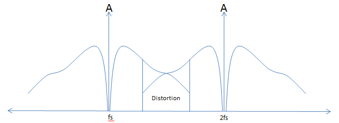
Figure 4: Under Sampled Unfiltered Speech Spectrum
Figure 4 above shows a speech waveform sampled at a frequency fs, which is less than twice the highest frequency content of the original signal. You can see that the area of aliasing (distortion of the speech) is significant. If we were to continue to increase the sampling frequency the distortion would diminish however the bandwidth required to transmit that signal would also increase. As with all things engineering there is a compromise. The increased sampling frequency helps to remove aliasing however it comes at a higher required bandwidth and a higher required processing performance to digitally filter the signal, compress the signal and transmit the signal.
To avoid this aliasing the original signal must be filtered in the analog domain to ensure that there are no components of that signal above half the desired sampling frequency. The ideal low pass filter response can be seen in Fig 5.
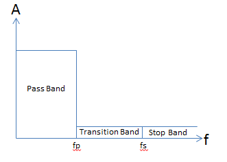
Figure 5: Ideal Filter Response
The gain of the filter in the pass band should be constant. Ideally the transition band shall have an infinitely steep roll off at frequency fp resulting in the transition band being infinitely small. Finally, the stop band would have a gain of zero � i.e. any signal that had a frequency component above fs would be completely filtered out. There are many types of filters, Butterworth, Elliptical, Chebyshev, inverse Chebyshev and so on. It�s not the aim of this paper to discuss the merits of each. However there are many tools out there now that can design your filter for you such as Webench or Simulation tools such as Matlab.
By applying the ideal filter response to the original unfiltered speech spectrum, the result would be a signal as shown in figure 6 below. The signal in the pass band of the filter is unaffected but the signal in the transition band and the stop band is no longer there. We have now cut-off the analog signal at 3KHz
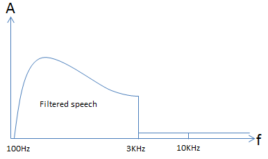
Figure 6: Filtered Speech Response
In the analog domain it is not possible to get close to the ideal filter response. The typical response of an analog two pole filter can be seen in fig 7 below. If the filter is designed to have a cut-off frequency of 3KHz (fp)then a two pole filter attenuates by 12dB by the time the cut off frequency doubles. That results in a 15dB attenuation at twice the cut off frequency. It is possible to design filters with more than two poles. Each pole adds 6dB of attenuation at twice the cut off frequency however, each additional pole has the effect of reducing the phase margin and can result in an unstable filter.
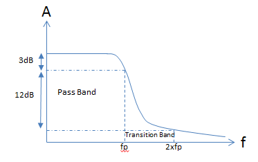
Figure 7: Two Pole Filter Response
Figure 8 shows how filtered speech would look like after being filtered by a two pole filter.
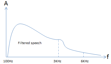
Figure 8: Two Pole Filter Speech Response
To sample this signal and not cause aliasing then the sample rate must be at least 6KHz. This is the theoretical minimal sampling frequency. In reality the sampling frequency should be higher. An ideal filter has a brick response but in reality a filter has a sloped response so you need to add in as much margin as practically possible. This is why the sampling rate is at 8KHz in most telecom systems.
By sampling we know that will create a mirror image of the waveform around the sampling frequency. This can be seen in fig 9 below.
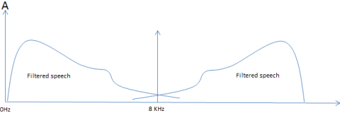
Figure 9: Sampled Filtered Speech Response
The analog signal has been filtered with a cut-off frequency of 3KHz and sampled at 8KHz. It can be seen that the area of aliasing (distortion on the speech) is almost non-existent. Increasing the sampling frequency would have little effect on the distortion. By sampling the filtered analog signal we have reduced the bandwidth and processing performance that would otherwise be required to compress and transmit the speech.
Digital filters
At this point it is worth briefly discussing digital filters. In the analog domain it is impractical to go beyond a six or maybe an 8 pole filter. The main reasons are instability in the circuit and the tolerances of resistors, capacitors, amplifiers, etc. make it almost impossible to design a stable and reproducible filter. This however is not the case in the digital domain. There are two main types of digital filters:
- IIR � Infinite Impulse Response filter.
- FIR � Finite Impulse Response filter.
Without going into to any details on implementation, the FIR filter is typically the choice of filter in the digital domain as it is inherently stable regardless of the number of poles in the filter. Using the FIR filter it is possible to get close to the ideal filter response shown earlier.
It is possible then in the digital domain to design a filter with a very small transition band and filter out and signal above 8KHz. By applying the ideal filer response to the sampled filter signal shown in fig 9 we would get a signal as shown in fig 10. There will be a small area of distortion near the sampling frequency due to aliasing and the digital filter response however, that will have little impact on the quality of speech.
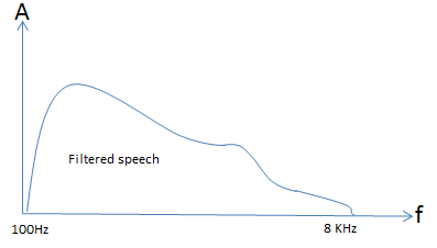
Figure 10: Digitally filtered Sampled Speech
Analog to Digital conversion
We have talked about filtering and sampling the signal but how is the conversion from the analog to digital domain accomplished.
There are several different architectures of an Analog to Digital Converters (ADC�s). Below are a few of the most common ones
- SAR � Successive Approximation Register � This architecture lends itself to low power, low area of silicon (hence low cost), very accurate and typically offer up to 16 bit outputs.
- Pipelined � This ADC operates as a parallel architecture which has the effect of using more power, more silicon area (increased cost), increased latency however can sample at much higher rates than a SAR � up to 1GHz sampling rates are practical.
- Flash � This architecture has a bank of comparators and is somewhat analogous to the pipelined architecture as it works in a parallel mode. This type of architecture is used for very high sampling rate � beyond 1GHz sampling rate is easily achievable but the number of output bits are typically limited to 8 or maybe 10 bits.
- Delta-Sigma � this is sometimes referred to as a single bit ADC. It is very accurate and can have output bits in the range of 24 or even 28 bits - it gives excellent resolution. The sample rate however is typically less than 100 KHz.
Sampling speech at 8 KHz, a SAR ADC is still typically the most common used. In the last 15-20 years delta sigma ADC's have become more prevalent for audio and speech sampling and are found in some voice applications.
How does an ADC work?
The description below is a very brief explanation of how a typical SAR ADC would work. For a much more in-depth look at the various architecture, this paper from Analog Devices gives an excellent overview.
A SAR ADC has a reference voltage that it uses to compare against the incoming signal � let�s assume 5v. If the ADC has a 12 bit output for each sample then the smallest analog input voltage that would cause the ADC to generate a new output value would be 5v/2N �Where N is the number of bits - 5v/4096 which is 1.22mV. Every 1.22mV of change causes the ADC output to change by a Least Significant Bit (LSB). You can see that this is a linear relationship between the input voltage swing and the output of the ADC.
Now we have filtered and digitized the voice we now have to transmit it. Taking the raw samples and transmitting them is certainly the most obvious method. The bandwidth to do this would be 8000x12 � sample rate x number of bits � 96kbps. However there are methods that can be employed to reduce the bandwidth and still have high fidelity voice calls. The generic term for the function to reduce the bandwidth is a CODEC � Compression/Decompression.
CODEC�s
There are many CODECs employed in a VoIP network. All CODECs developed in the past 20 years or so rely heavily on the advancements in processing performance of the latest DSP�s. These algorithms are mathematically very intensive and were only made practical as DSP�s from companies like Texas Instruments become mainstream.
G.711 CODEC
The G.711 codec is one of the most widely spread codecs in use today. G.711 was first introduced in the early 70�s and was very easy to implement, didn�t take much processing power and could be implemented in the analog domain in the early years of telecom. G.711 employs something called companding.
With a phone call, ideally you would like to amplify the voice more when someone is whispering than when someone is talking loud or shouting. The best way to do this is to use a non-linear sampling method, referred to as companding.
Let�s pictorially look at the effect of non-linear sampling.
Figure 11 below shows two waveforms. The red waveform is the original speech plotted in the time domain. Once the signal has been companded it would look like the green trace � again plotted in the time domain. It can be seen that the lower amplitude signals have effectively been amplified and the higher amplitude signals have been largely untouched. This has the effect of reducing the dynamic range of the signal but the benefit is the amplified low level signals. This is exactly what you would want for speech � amplifying the signal when someone is whispering and leaving the higher amplitude signals untouched.
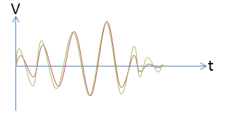
Figure 11: Companded Speech
There are three potential implementations of non-linear sampling.
- Using a non-linear gain amplifier.
- Using a non-linear ADC.
- Using a DSP or processor and implement the algorithm in the digital domain.
Using a DSP or processor is exclusively used these days as digital processing has become much more powerful and memory has been getting cheaper and cheaper. Non-linear designs in the analog domain are extremely difficult to consistently reproduce and are susceptible to component tolerances, temperature, physical layout, noise, etc. Once digitized the samples are much more immune to noise.
There are two types of logarithmic sampling methods, u-law and A-law. u-law is primarily used in North America and Japan and A-law is used elsewhere. Both u-law and A-law employ similar techniques and both result in an 8 bit digital value for each sample. A-law gives slightly better quantization at lower levels which results in slightly better quality of speech.
Below is a table showing the uncompressed linear samples and the corresponding A-law compressed samples. Logically you look for the most significant �1� in the uncompressed sample and you encode the position into a three bit value. The four most significant bits after the most significant �1� are untouched, these bits are represented by �wxyz�. Any bits blow these four are thrown away. The Most Significant Bit (MSB) of the uncompressed stream is a sign bit and directly translates to the sign bit of the compressed stream, represented by �S�.
| Linear 13 bit Sample | Compressed 8 bit Sample |
|---|---|
| S0000000wxyz | S000wxyz |
| S0000001wxyz | S001wxyz |
| S000001wxyz�a | S010wxyz |
| S00001wxyz�ab | S011wxyz |
| S0001wxyz�abc | S100wxyz |
| S001wxyz�abcd | S101wxyz |
| S01wxyz�abcde | S110wxyz |
| S1wxyz�abcdef | S111wxyz |
Table 1: G.711 Codec Samples
u-law works in a very similar fashion.
There are many newer and more advanced codecs than G.711. These CODECs are much more complicated and require a significant amount of processing power. The digitally sampled voice can be compressed down to 8kbs and in some cases even lower and yet still give good quality speech. Other wideband codecs such as G.729 are sometimes referred to as High Definition CODECs. These codecs take speech that is sampled at 16 KHz giving much higher frequency content and a much higher fidelity.
We have explored how speech is sampled and how to compress it yet still retain toll quality speech. Now we will look at how the compressed speech is actually transmitted via the internet.
Internet Protocols
What protocol is best for transmitting real time speech?
There are many different protocols that can run over the Internet. Below is a list of some of the common protocols currently running over the internet.
| Acronym | Definition | Purpose |
|---|---|---|
| TCP | Transmission Control Protocol | guarantee delivery |
| IP | Internet Protocol | data oriented |
| UDP | User Datagram Protocol | fire-and-forget |
| ARP | Address Resolution Protocol | finding an address |
| RARP | Reverse Address Resolution Protocol | finding an address |
| BOOTP | Bootstrap Protocol | finding an address |
| DHCP | Dynamic Host Configuration Protocol | adding devices to a network |
| BSD | Berkeley Socket | connecting to the internet |
| ICMP | Internet Control Message Protocol | error message generation |
| IGMP | Internet Group Management Protocol | manage IP multicast groups |
| PPP | Point-To-Point Protocol | direct point-to-point connection |
| SLIP | Serial Line Internet Protocol | direct point-to-point connection |
| DNS | Domain Name System | translate host name to address |
| FTP | File Transfer Protocol | transfer files point-to-point |
| TFTP | Trivial File Transfer Protocol | FTP, but for smaller files |
| RIP | Routing Information Protocol | routing internal networks |
| RTP/RTCP | Real-time Transport (Control) Protocol | send audio/video over internet |
| Telnet | Terminal Emulation | remote access |
| HTTP | Hypertext transfer Protocol Server | publish/retrieve web pages |
| SNMP | Simple Network Management Protocol | manage/monitor client status |
| SMTP | Simple Mail Transport Protocol | send email over internet |
| POP3 | Post Office Protocol-3 | retrieve email over internet |
| SNTP | Synchronized Network Time Protocol | network clock synchronization |
| PTP | Precision Time Protocol (aka IEEE1588) | deterministic synchronization |
| NAT | Network Address Translation | network privacy |
| SSLS | Secure Sockets Layer | secure communication |
| IPSec | Internet Protocol Security | virtual private network |
| IKE | Internet Key Exchange | security key/certificate sharing |
Table 2: Internet Protocols
It�s important to know the different requirements placed on a network and a protocol when transmitting data or speech.
Reliability � this may seem a little counter intuitive but speech does not require as a reliable connection as data. You may be thinking that as data and voice are both being sent over the internet so the connection is the same. The physical connection is the same, Ethernet, T1 lines, switches, routers, etc. but the protocol need not be the same. This is a very important concept to grasp. There are many protocols as can be seen in table 2, that are developed with particular functions and applications in mind, however these protocols can all run over the exact same physical path.
TCP v UDP
Most are familiar with a term called TCP which stands for Transmission Control Protocol � this is how data is transmitted over the internet. However less well known is a protocol called UDP (User Datagram Protocol). Let�s look at the main differences between these two protocols and the advantages and disadvantages of each when transmitting real time data.
- The TCP protocol was designed for data transmission and as such it has a built in mechanism for performing error checking. This means that if a packet does not arrive or is corrupted in some manner then there is a mechanism for retransmitting the packet. This is essential for data but has significant consequences for speech. Retransmission of speech would cause significant delay and make a conversation impossible. UDP packets, although having a checksum field do not mandate the use of this field. UDP packets use a "fire and forget" type of transmission, there is no re-transmission of corrupt or lost packets - keeping the delay to a minimum is key for real time communication.
- TCP has provisions to check the order of the packets received. If packets are received out of order they are buffered and reordered. The downside of the reordering process is the additional delay, this is not an issue with a data transfer but the associated delay has a significant impact on real time data communication. UDP packets have no field defined for packet numbering, there is no provisions for reordering packets when using UDP.
- TCP sets up a point to point connection between the source and destination. This is done by the source requesting a connection to the destination and the destination sending back an acknowledgement message. This does not set up a particular path through the network, rather it just defines that the source and destination are the only two nodes in the connection. TCP cannot do multicast, an absolute necessity for voice if you want to do a conference call or even 3-way calling. UDP does not set up a connection between the source and the destination but rather performs a �fire and forget� type of transmission. This means that it is possible to have multiple nodes in a call.
As can be seen TCP is not a good choice for real time data � video, voice, etc. UDP is a much better option.
Packet formats
Before going on to look at the formats of the UDP packet we first must look at the RTP packet. The RTP packet is the actual packet that encapsulates the compressed speech samples.
RTP Packet Format
Below is a table indicating the different fields that make up the RTP packet.
| 32 bit word | Function |
|---|---|
| 0 | Control info + sequence number |
| 1 | Timestamp info |
| 2-3 | Synchronization & Contributing Source Identifiers |
| 4 | Profile specific extension headers ID�s and lengths |
| 5 | Extension Header ID |
| 6 | Extension Header |
| 7 - onwards | Payload |
Table 3: RTP Packet Format
- Control info and sequence number � These 32 bits are split into two 16 bit fields. The first 16 bits hold various control parameters and the second 16 bits hold the sequence number of the packet. We said earlier that voice does not require re-sequencing of packets as it adds to delay. The 16 bits that form the sequence field is included and leaves the choice to re-sequencing packets up to the application layer.
- Timestamp � This 32 bit field holds a timestamp for each packet. For packets that transfer speech samples this field can be used to transmit the sample rate that the speech was sampled at � typically 8KHz.
- Synchronization & Contributing Source Identifiers � These two 32 bit fields hold the source identifier, if the stream holds sources form multiple streams then this would be defined in the Contributing Source field.
- Extension Header ID � This 32 bit field is optional and is only included of extension headers are used � this field defines the header type and length.
- Extension Header � This 32 bit field is optional and is the actual header extension defined by the Extension Header ID.
- Payload � This is the actual data to be transmitted, in this case it�s the digitally compressed voice samples.
UDP Packet format
The table below shows the format of a UDP packet.
| 32 bit word | Function |
|---|---|
| 0 | Source Port |
| 1 | Destination Port |
| 2 | Length |
| 3 | Checksum |
| 4 - onwards | Payload |
Table 4: UDP Packet Format
- Source Port � This 32 bit field is the source address of where the data came from. Earlier we said that there is no connection setup as there are no requirements for retransmission of missed or corrupt packets. Even though this field is not necessary it is typically filled with all �0�s.
- Destination Port � This 32 bit field is the address of where the data is going.
- Length � This 32 bit field is essential so the receiving side knows how much data to expect in a packet.
- Checksum � This 32 bit field can be used to see if the data has been corrupted during the transmission. As no retransmission of corrupt data is required for VoIP then this field has no significance.
- Payload � This is the RTP packet.
As you can see it is a very minimalistic and simple packet format, exactly what you would want to minimize bandwidth. The source port and checksum fields are not required but provisions are made for future growth. If IPv6 rather than IPv4 is used then the checksum block is required.
The UDP packet is further encapsulated in an IP packet.
IP Packet Format
There are two main formats for an IP packet. IPv4 is a standard that has been used since the concept of IP packets. When the concept of connected devices with an IP address for everyone of those devices was first envisaged, provisions for 4.3 Billion addresses seemed like a safe bet. In the past couple for years due to the proliferation of wireless technology we have easily surpassed this. To address this issue, IPv6 was developed. The main difference between IPv4 and IPv6, that has an effect on bandwidth is the source and destination IP addresses. These two fields have been increased from 32 bits to 128 bits. With IPv6 there are 2^128 source and destination addresses.
The format of a IPv4 IP packet can be seen below.
| 32 bit word | Function |
|---|---|
| 0 | Control info + packet length |
| 1 | Identification info, flags and fragment offset |
| 2 | Control + data checksum |
| 3 | Source IP address |
| 4 | Destination IP address |
| 5 - onwards | Payload |
Table 5: IP Packet Format
- Control Info and packet length � This 32 bit field defines the type of protocol used (IPv4 or IPv6), type of service, header length and finally the packet size.
- Identification info, flags and fragment offset � This 32 bit field is almost exclusively used to re-assemble fragmented packets at the destination.
- Time to live, protocol + data checksum � This 32 bit field defines how long a packet is valid in the network before being discarded. The protocol the packet is intended for at the destination and finally a checksum for the packet to determine if any bits in the stream were corrupted during transport.
- Source IP address � This 32 bit field identifies the IP address of the source.
- Destination IP address � This 32 bit field identifies the IP address of the destination.
- Payload � This is the actual data to be transmitted, in this case it�s the UDP packet.
Payload size v Delay
The packet formats described above give an indication of the overhead for transmitting data. As usual with all things in engineering there is a compromise. The larger the actual size of the source data we want to send then there is a smaller percentage of the bandwidth used up for the header information as this is fixed. However, the larger the data packet sent for a real time voice application such as VoIP then the longer the delay. There has to be a compromise between the size of the payload and the delay incurred by the packet size.
There are many delays incurred when transmitting data in an IP network - capturing the data, compressing the data, formatting the packet, delays through the network (switches and routers), receiving the packets, decompressing the samples and then converting them back to the analog domain. A delay approaching 200ms from mouth to ear makes a conversation very difficult to hold. To keep the delay to a minimum typically 20-30ms worth of data is sent at a time.
Bandwidth Required
Let�s determine the actual overall bandwidth required for a typical VoIP call. Let�s assume G.711 encoding which results in a 64Kbits per second compressed data rate. Let�s also assume we are sending 20ms worth of data at a time.
By sending 20ms of data at a time, the result is 50 Internet Packets to be sent in one second � make a mental note of that.
In an RTP packet there are eight 32 bit words in the header information. This equates to 32 additional bytes for every packet.
The RTP packet is encapsulated in a UDP packet. A UDP packet has four 32 bit words in the header which results in an additional 16 bytes for the UDP packet.
The UDP packet is encapsulated in an IP packet, let�s assume IPv4 is used which gives an overheard of five 32 bit words for the header � so an overhead of 20 bytes.
Total overhead per IP packet is culmination of the overhead of the RTP packet, the UDP packet and the IP packet which is 68 bytes. Now, we said that there are 50 packets sent every second, so an additional 3400 (50x 68) bytes are sent just as header info. 3400 bytes per second in overhead data equates to 27.2Kbits per second.
So the total bandwidth for a VoIP call is the sampled data rate + 27.2Kbits**. This can be seen in the CODEC summary table.
** The application may add some extra in band control information, IPv6 may be used, the IP packet may be encapsulated in a higher order protocol, more than 20ms of voice may be packetized at a time, even the physical medium could add bandwidth if something like 8b10 encoding is used. This 27.2Kbits per second is a theoretical minimum and in practice it�s safe to add a 20% overhead on top of this number.
Conclusion
The sampling theorem and voice compression via the the G.711 Codec have been around for many years, they are very well understood and have been optimized over the years. The advent of cellular communication in the late 80's spurred significant research and development in the area of speech compression and as a result there are a plethora of CODECs available each with their own unique advantages. VoIP has become mainstream in the past decade or so as bandwidth over the internet has increased allowing for toll quality phone calls, in addition using the same technology to transmit data and voice has facilitated the integration of these services and has brought about the advancements in unified communications.
This paper has focussed on what happens when you pick up the phone and call. It has explained the need to filter and sample the analog voice, it has explained how that is accomplished, the types of codecs and how they are implemented and finally how the data is formatted and sent via the internet. This paper has brought the major functions of making a VoIP call together and has endeavoured to explain how and why the various technologies and functions come together.